Machine Learning Basics
pedagogic talk mainly based on
Nanotemper Technologies · Munich · 10 June 2016
F. Alexander Wolf |
Institute of Computational Biology
Helmholtz Zentrum München


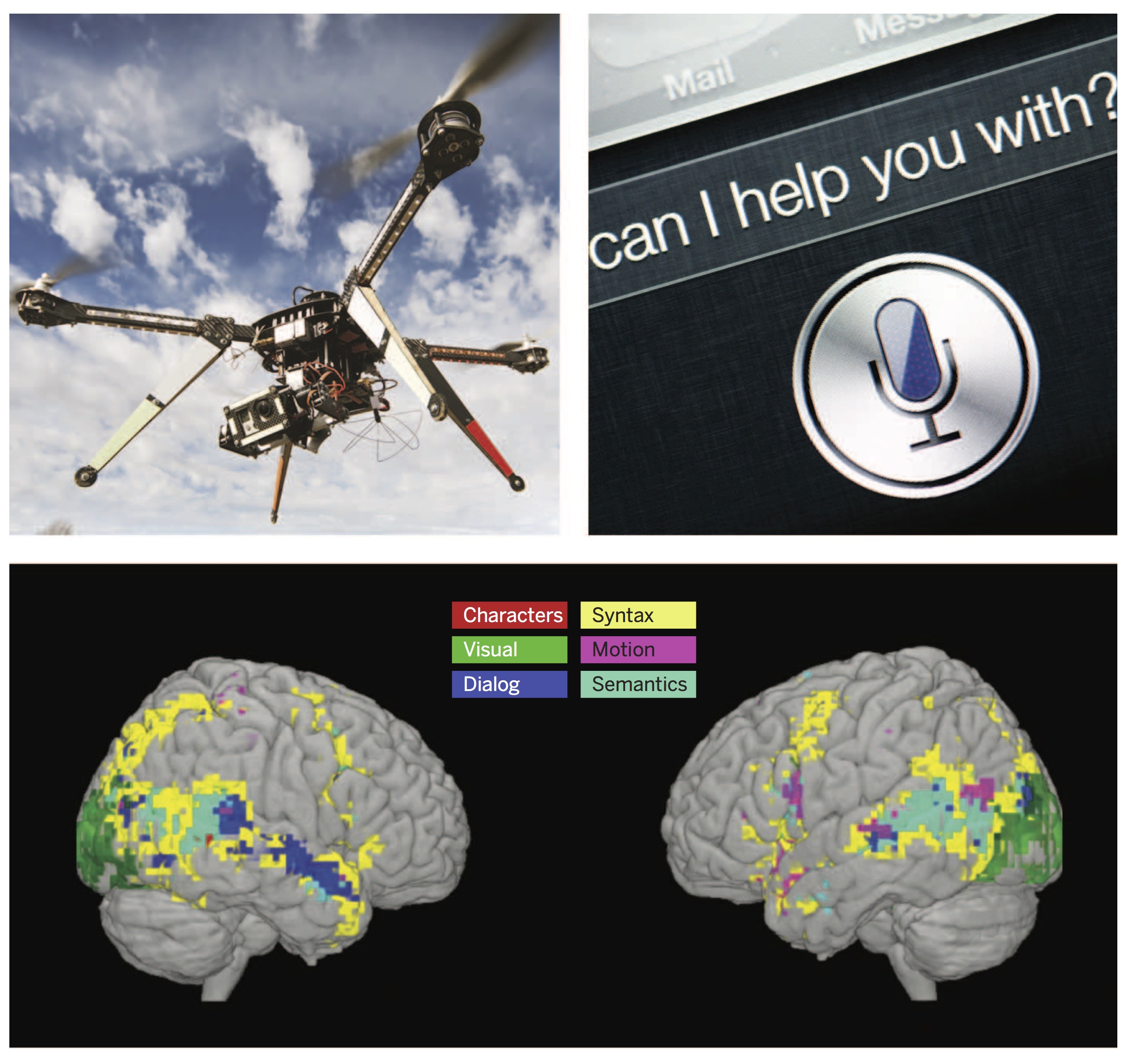
Machine learning in robotics,
natural language processing, neuroscience research,
and computer vision.
What is Machine Learning?
It's statistics using models with higher complexity.
These might yield higher precision but are less interpretable.

What does Machine Learning?
- Estimate a functional relation f:X→YX↦Y from data D={(xi,yi)}Ni=1 (supervised case).
- Estimate similarity in the space X from data D={xi}Ni=1, xi∈X (unsupervised case).
Comments
- Estimation based on data is referred to as learning.
- Also the supervised case requires learning similarity in X.
Classification example

Learn function f:R28×28→{2,4}.
In which way are samples, e.g. for the label y=2, similar to each other?

▷ Strategy: find coordinates = features that reveal the similarity!
▷ Here PCA: diagonalize the covariance matrix (x⊤i⋅xj)Nij=1.
A simple model: k Nearest Neighbors
Model function ˆf: estimator ˆyx for Y given X=x ˆyx=ˆfD(x)=Ep(y|x,D)[y]=1k∑i∈Nk(x,D)yi


A simple model: k Nearest Neighbors
Model function ˆf: estimator for Y given X=x ˆyx=ˆfD(x)=Ep(y|x,D)[y]=1k∑i∈Nk(x,D)yi Probabilistic model definition reflects uncertainty p(y|x,D)=1k∑i∈Nk(x,D)I(yi=y)
- Overfitting and Bias-Variance tradeoff: the lower the variance, the higher the bias.
- Is non-parametric, so no learning of parameters.
- Assumption: Euclidean distance is good similarity measure for x.
- Curse of dimensionality: does not work in high dimensions.
Another simple model: linear regression
Estimator for y given x ˆyx=ˆfθ(x)=Ep(y|x,θ)[y]=w0+x⊤w Probabilistic model definition p(y|x,θ)=N(y|ˆyx,σ),θ=(w0,w,σ) Estimate parameters from data D θ∗=argmaxθp(θ|D)
- Parametric, parameters θ have to be learned.
- High bias due to linearity assumption, but works in high dimensions, and is easily interpretable.
Learning parameters
Estimate parameters from data D
θ∗=argmaxθp(θ|D,model,beliefs),Optimization
assuming a model and prior beliefs about parameters.
Now
p(θ|D)=p(D|θ)p(θ)/p(D).Bayes′ rule
Evaluate: assume uniform prior p(θ) and iid samples (yi,xi)
p(θ|D)∝p(D|θ)=N∏i=1p(yi,xi|θ)∝N∏i=1p(yi|xi,θ)
Linear regression: logp(θ|D)≃∑Ni=1(yi−ˆfx1)2 ▷ least squares!
Learning parameters: robot example

Deep Learning: Neural Network Model

A Neural Network consists of layered linear regressions (one for each neuron) stacked with non-linear activation functions ϕ.
P(y|x,θ)=N(y|v⊤z(x),σ2)z(x)=(ϕ(w⊤1x),…,ϕ(w⊤Hx))
- Deep learning means many layers.
- In each hidden layer, combine weights wi to matrix W.
Deep Learning: Idea
- V1 is arranged in a spatial map mirroring the structure of the image in the retina.
- V1 has simple cells whose activity is a linear function of the image in a small localized receptive field.
- V1 has complex cells whose activity is invariant to small spatial translations.
- Neurons in V1 respond most strongly to very specific, simple patterns of light, such as oriented bars, but respond hardly to any other patterns.
Deep Learning: Convolution Layer
- discrete convolution of functions ft and wt, t∈{1,2,...,D},˜f=∑τwt−τfτ=Wf,˜f,f∈RD where Wtτ=wt−τ, W∈RD×D.
▷ Instead of D2, only D independent components.
Natural extension: sparsity
-
demand: wt−τ!=0 for |t−τ|>d
[usual property of kernels: e.g. Gaussian Wtτ=e−(t−τ)22d2]
▷ Instead of D2, only 2d nonzero components. ▷ Statistics ☺!
Deep Learning: Convolution Layer
(arrows represent arbitrary values)

(arrows: same values across receptive fields )

Deep Learning: Why is convolution useful?
Consider an example (d=1)
W=(⋱−110⋱⋱0−11⋱) ⇔ ˜ft=ft−ft−1,
that is, f =

↦˜f =

▷ Simple edge structures revealed! Just as the simple cells in V1!
Deep Learning: Pooling layers
Assumption
- In most cases, classification information does not depend strongly on the location (index t) of a pattern. That is, the presence of a pattern is more important than its location.
- In many cases, our only interest is the presence or absence of a pattern.
Max-Pooling Layer
- implement local translational invariance
- Just as complex cells in V1.
![]()
![]()
Deep Learning: Convolutional Neural Network

- Read input f.
-
Convolution stage
˜f(k):=W(k)f,
where W(k) is one of K convolution kernels, k=1,...,K. - Detector stage ˜f(k)t:=ϕ(˜f(k)t+b) where ϕ is an activation function, b a bias.
- Pooling stage ˜f(k)t:=maxτ∈[t−d,t+d]˜f(k)t
Deep Learning: Comments
-
Receptive field grows and
more and more complex features are constructed in each layer.
![]()
-
What to generally learn from deep learning?
Convolutional networks are so successful because they efficiently encode our (correct) beliefs about the structure of certain data (translation-invariant, simple local features, complex features from simple features).
▷ Understand the similarity structure of your data and use a model that reflects it!
Summary
- Machine Learning ist Statistics with models of higher complexity.
- It's all about similarity in the data space.
- Two simple examples: kNN and linear regression
- Learning is Bayes rule followed by an optimization.
- Deep Learning: very successful way of understanding and exploiting the similarity structure of e.g. image data.

Thank you!


